What is concept drift?
Concept drift is a problematic phenomenon in which a predictive model’s performance degrades over time due to changes in its environment. To illustrate, a model is trained on historical data and is used to make predictions on unseen data. This model maps the relationship between the input features and the target variable. However, over time, this learned relationship is bound to change. As a result, the mapping learned during training no longer matches the relationship between the input features and the target variable for deployment data. In other words, the environment has changed, yet the model is unaware of these changes and thus becomes outdated.
Drift can have a far-reaching, detrimental impact on operational and strategic business decisions. In the context of demand forecasting, which we will use as a running example throughout this article, this can result in inaccurate inventory planning along with potential cascading effects across the supply chain. Additionally, given that forecasts play a central role in long-term planning as they are used to prepare for seasonal spikes and determine future capital expenditures, their accuracy is of crucial importance.
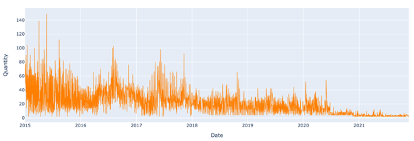
Let us take for example a model that is used to predict sales quantities for the time series below. The model is trained using data from the beginning of 2015 until the end of August 2019 and is used to make predictions from then onwards. As can be seen below, sales quantities sharply dipped in July 2020. Given that the model has not been trained during this period of sustained decrease in sales quantities, its performance will likely degrade.
How quickly can Model Drift happen?
Let us now look at the different rates at which drift can emerge over time.
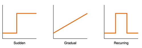
- Sudden: This shift occurs abruptly due to unforeseen circumstances. A clear example is COVID-19 and the lockdowns that caused a drastic change in consumer behaviour and demand.
- Incremental/Gradual: The transition from one distribution to another unfolds over a long period here. An example of this is rising temperatures across the globe over time as a result of global warming.
- Recurring/Seasonal: For this type, patterns seen in the past reappear over time. For example, increases in consumer demand during Black Friday and Christmas due to the repeating nature of these events. Since recurring drift is more predictable than other drift types, its effect can be mitigated by taking seasonality into account as an input feature during model training.
How to solve Model Drift?
Approach 1: Regular Retraining
As static models are particularly at risk of drift, regularly updating a model can arm it against the threat of decreased model performance over time. By updating the model at regular intervals using new training data, one can ensure that the model continuously learns new patterns in its environment. The training frequency is decided based on the stability of the environment in which the model is operating.
For instance, a model designed to predict sales quantities would likely require a different retraining interval than a model designed to predict stock prices. Consequently, this decision should be guided by prior analysis of historical data.
Approach 2: Drift Monitoring and Detection
Monitoring the predictive performance of a model can be used to ensure a model’s continued reliability. Users can get notified when a model’s performance drops below healthy levels and thus can take remedial actions in due time. While there exists a multitude of methods that detect drift, they vary in complexity and accuracy. We demonstrate a method that strikes a balance between both, statistical process control (SPC). This quality control method is frequently adopted in manufacturing environments to maintain product quality by monitoring process variation. For our purposes, the relevant process is a model’s residuals.
SPC assumes that all processes are subject to variance. Moreover, variance can be due to chance or an assignable cause. One-off, random variations in the process are referred to as noise, not drift. Given that we are not interested in detecting this phenomenon as it is inherent to the process and is unalarming, the drift detection algorithm should be resilient towards it. On the other hand, we are interested in detecting persistent changes in residuals over time as they are an indicator of drift. Therefore, points of interest are consecutive points that fall outside a lower or an upper bound. These bounds are calculated using the mean and standard deviation. Please refer to the code block below for a reference of how SPC can be programmed.
class SPC():

   def __init__(self, delta: int, window:int = 20, minPoints:int = 10):
       self.delta = delta
       self.window = window
       self.minPoints = minPoints
       self.pointList = []
       self.sigma = 0
       self.upperBound = 0
       self.lowerBound = 0
       self.processMean = 0


   def calculate_stats(self, datastream: np.array) -> None:
       """Calculate the mean, standard deviation, and bounds of the datastream.

       Args:
           datastream (np.array): Datastream to calculate stats for."""

       self.processMean = datastream.mean()
       self.sigma = datastream.std()
       self.upperBound = self.processMean + self.delta * self.sigma
       self.lowerBound = self.processMean - self.delta * self.sigma

   def add_element(self, datastream: np.array) -> List:
       """Test each datapoint inside datastream against upper and lower bound and store results in pointList.
       False refers to no drift and True refers to drift.

       Args:
           datastream (np.array): Data to be tested. Should be a 1D array.

       Returns:
           pointList (List): List populated with booleans based on testing condition for each point in datastream.
       """
       self.calculate_stats(datastream)
       self.pointList = np.logical_or(datastream <= self.lowerBound, datastream >= self.upperBound)
       return self.pointList

   def detected_change(self) -> bool:
       """Test whether a certain number of points fall outside upper and lower bound within a certain number of days.


       Args:
           : bool: True if drift is detected, False if not.

       Returns:

           drift_comparasion (np.array): Populated with boolean values indicating whether drift was detected.


           drift_region (tuple): Populated with drifting residuals indices.
       """
       num_errors = np.sum(np.lib.stride_tricks.sliding_window_view(self.pointList, window_shape=(self.window,)), axis=1)
       drift_comparasion = num_errors >= self.minPoints
       drift_region= np.nonzero(drift_comparasion)
       return drift_comparasion, drift_region
A few parameters in the code above should be tuned by the user. First, a delta parameter which is used to calculate the upper and lower bound. The larger this parameter, the further away from the mean the drifting points need to be to be classified as drift. Moreover, a window parameter which restricts the number of days in which drifting points can be detected to a limited time window. This parameter ensures that the drifting points are close enough, for if they are too far apart, they are noise and not drift. A larger window reduces false negatives at the expense of an increased risk of false positives. Lastly, the minPoints parameter refers to the number of data points that should fall outside the upper and lower bound for drift to be detected. The larger the value, the lower the risk of capturing false positives. Since there is a tradeoff between accuracy and false alarms when tuning these parameters, experimenting with different values is encouraged to find ones that fit the use case and the user’s risk tolerance.
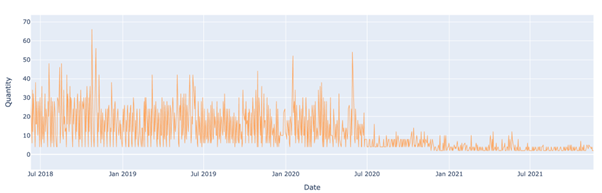
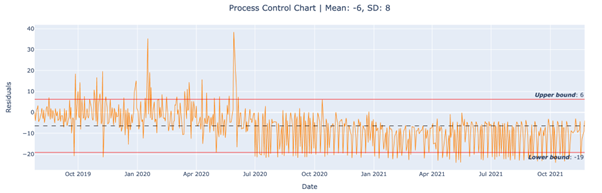
To put SPC to the test, a random forest regressor model was trained to predict sales quantities from August 2018 onwards for the same time series we saw earlier. The algorithm detects drift if, in a window of 30 days, 10 days are beyond the upper or lower bound. Drift was indeed detected when it started occurring in July 2020 as can be seen below. Also, the preceding spikes were not detected, as they should be given that they are noise - this is ensured by tuning the minPonts parameter.
In practice, the mean and standard deviation of the test set should be used as a baseline to which residuals of a deployed model are compared. This is recommended as one would like to discover whether a model’s performance has changed in comparison to what it was tested on during development.
Conclusion
We uncovered what drift is and why it is problematic. We also discussed different rates at which drift could occur and demonstrated how a model's performance can be tracked using SPC. If interested in further resources, the reader is referred to the following Github repository for the full code along with other drift detection algorithms. This repository is part of the writers’ master’s thesis project titled “Impact of Concept Drift on Predictive Performance in Time Series Forecasting” in collaboration with element61.