Introduction: Why do we care about data modeling best practices
Power BI is not only a tool to create fancy visualization, but it is an interactive business intelligence reporting tool where the primary focus is to provide the end users with the best possible way to create data-driven insights at the enterprise level at scale. It is thus imperative that the reporting platform is performant, capable of performing complex analytical calculations, of holding large historical data, and of providing self-service and many other critical BI features. One of the fundamental pillars to achieve this aim is to have in place the best data modeling practices suitable for our Power BI datasets. Let’s get started…
Star Schema is your friend
Like any other OLAP model (i.e. Online Analytical Platform), Power BI works best with a star schema design, where a Fact, its measures, and transactional dates have foreign key references towards the dimensions, the dimensions which we need for filters, slicers or KPI calculations. Star schema is the easiest method to present data intuitively with high performance and additional functionality used in a data warehouse concept. A simple star schema has been depicted below:
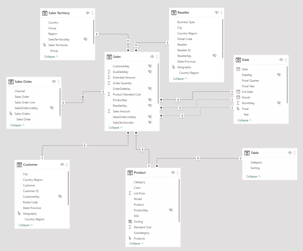
Figure 1 - A simple sales star schema
Avoid many-to-many and bi-directional relationship
Many-to-many relationships should be avoided at any cost. It multiples the value of measures and shows the wrong value for them. It also does not support the DAX-related () function. Although technically it can work with applying correct filters, it creates confusion for the end users, which might be difficult for maintenance. Typically, when we join 2 fact tables, which ideally should never be joined directly, many-to-many relationships occur. Below, we have a section covering how to join 2 fact tables.
Bi-directional relationships are required while working with:
a) one-to-one or many-to-many relationship,
b) if one slicer needs to filter data in another slicer,
c) analysis across multiple dimensions.
For a) one-to-one relationships, one scenario is when we have a fact table and a degenerate dimension: the relationship in most cases is one-to-one. Since the table size would almost be the same, the table direction would not really matter. But in another scenario, it is not recommended to use one-to-one relationships when row data spans across multiple tables. For many-to-many relationships, in any case,e it should be avoided.
For b), this use case is most common for the use of bi-directional filters, but some users are not happy with slicer values appearing and disappearing; we can instead apply a visual level filter to achieve the same result.
For c), we need to use this relationship type anyway, but a DAX function crossfilter() helps to reduce the impact. Bi-directional filters generate a greater number of queries in the backend, so having it in the model can lead to a negative performance impact – hence the recommendation to avoid it.
Role-playing dimensions
Role-playing dimensions are a very common phenomenon in dimensional modeling techniques where a single dimension needs to play multiple roles. An easy example is Date dimension which can be linked with the Order Date, Purchase Date, Sales Date and several other dates associated with the fact table. Another example is an employee, manager, supervisor etc. who all are essentially an employee.
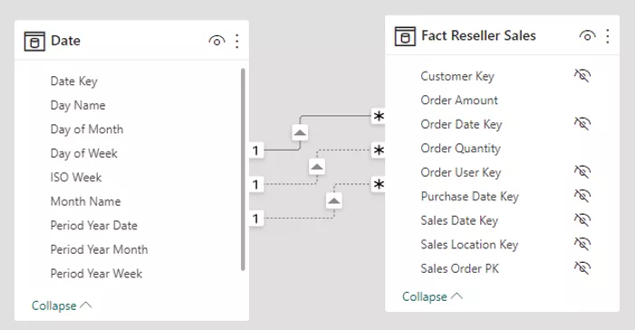
Figure 2 - Role playing dimension with inactive relations
Creating multiple date-dimension views can be an easy but ugly solution: it requires a lot of maintenance and awareness. So, one option is to use an inactive relation (as shown in Figure 2) between the fact and the dimension for all other date columns than the active relation date column and then, make use of the userelationship() DAX function to create a measure on the other date columns. There might be a requirement to create several measures based on these other date columns, in that case, we create calculation groups under which we can use this DAX function to automate the creation of these measures. If the requirement is also to filter or slice the data based on different dates, then inactive relationships would not solve the problem and you would have to go to the following option.
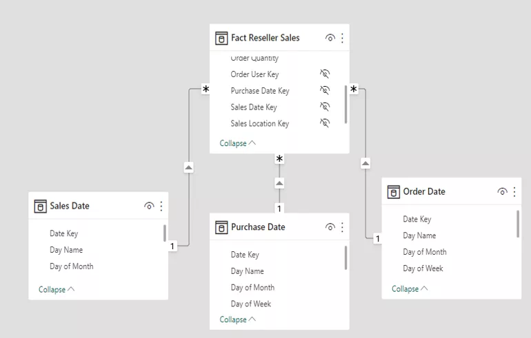
Figure 3 - Role playing dimension with duplicating via Power Query
And the easiest option is to duplicate your Date dimension or other role-playing dimension in Power Query editor without having to duplicate the view in DWH, as shown in Figure 3.
How to join multiple fact tables
Fact tables are often derived from different business transactions, resulting in them never having the same granularity. If it is required to use measures from more than one fact table, we end up getting a many-to-many relationship, but as mentioned, it should be avoided. We can create a shared dimension table which solves the many-to-many granularities problem, as shown in Figure 4. If we just want to show products sold vs. products invoiced against region, month, sales organization and then between our Sales Fact and Invoice Fact, we should use these three common dimensions which would solve the problem. If we really need to compare at the document level, we should have a shared dimension table where Sales order number and Invoice document number are linked to one another. Once the measures are created (even a dummy count measure can be created and then hidden), it would be possible to join both fact tables for the measures as well as for the columns.
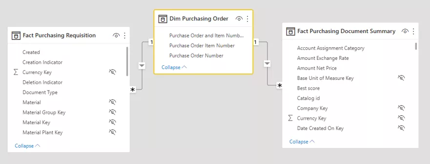
Figure 4 - Joining multiple fact tables with a common dimension to avoid many-to-many relations
Organize your Facts and Dimensions, as well as Measures
A good data model is easily comprehensible by a business user. We must follow the organization's standard naming conventions for our columns and measures. We need to hide any technical keys that are not meaningful to the business (an example is DWH surrogate keys). We always need to specify our dimensions and facts in the star schema. We also need to create explicit measures (the end users also want ‘analyze in Excel’) and preferably in separate folders/tables as shown in Figure 5.
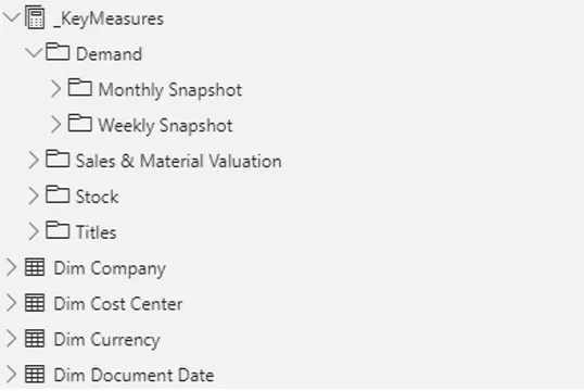
Figure 5 - Good naming convention is of paramount importance
Impact of calculated columns in your model
For complex calculations of a column, we recommend Roche’s Maxim of Data Transformation: “Data should be transformed as far upstream as possible and as far downstream as necessary”. So, if it is possible to create the calculated column in the data warehouse, let’s do that. If not, the next option is to do it in Power Query or, if that is also not possible, the last obvious option is that we use DAX calculations. Calculated columns are refreshed while refreshing the dataset and increase the size of the model, whereas measures are being calculated during the query time, hence more calculated columns degrade the performance of the overall model. Also, calculated columns in a fact table prevent it from being refreshed incrementally.
Enterprise Model vs. Local Model
In an enterprise, it is often a requirement to perform cross-functional reporting. For example, what is the revenue for product X against its manufacturing price or its purchasing price? Or, what is the stock left after production against the demand based on sales history? In such scenarios, we need to report on different business transactions which requires joining multiple fact tables from different functional domains. In the above example, we would have to join data between Sales, Finance, Purchasing and Inventory domains. The organization might want to create one “Enterprise Model” to fulfil its requirement or often different business units create their own “Local Model” to simplify their own needs. So the question is: which one should we use? Let’s try to solve this.
If the analytical reporting platform focuses on very few business processes, with limited number of report developers and users, it could be that having one centralized enterprise model is easier to maintain, which guarantees consistent KPIs. But if the organization is consisting of several large business departments and lot of complex unrelated business processes, it could become cumbersome to maintain one enterprise model. Maybe it would be a good idea to have one model per functional domain. The choice is also influenced by the governing model of your analytical platform.
So, it really depends. The pros and cons for both choices are depicted below.
| Enterprise Model | Local Model |
|
Pros:
|
Pros:
|
|
Cons:
|
Cons:
|
For more insights & research, visit the element61 Knowledge Base.


